The parameter table pattern is used to create parameters in a report, so that users can interact with slicers and dynamically change the behavior of the report itself. For example, a report can show the top N products by category, letting the users decide through a slicer if they want to see 3, 5, 10 or any other number of best products. The values available for a parameter must be stored in one or more disconnected tables, which do not have a relationship with any other tables of the same model. This chapter includes several examples with the parameter table, but this pattern has an even broader range of application.

In this pattern, we create the parameter tables by using DAX code. The Parameter feature of Power BI Desktop uses a similar technique. Indeed, the Parameter feature in Power BI Desktop creates a slicer tied to a calculated table computed with the GENERATESERIES function; it also creates a measure that returns the selected value of the parameter. This is the approach followed in this pattern. The main advantage of writing the calculated table manually in DAX is that it provides greater flexibility in the parameters to use.

Changing the scale of a measure

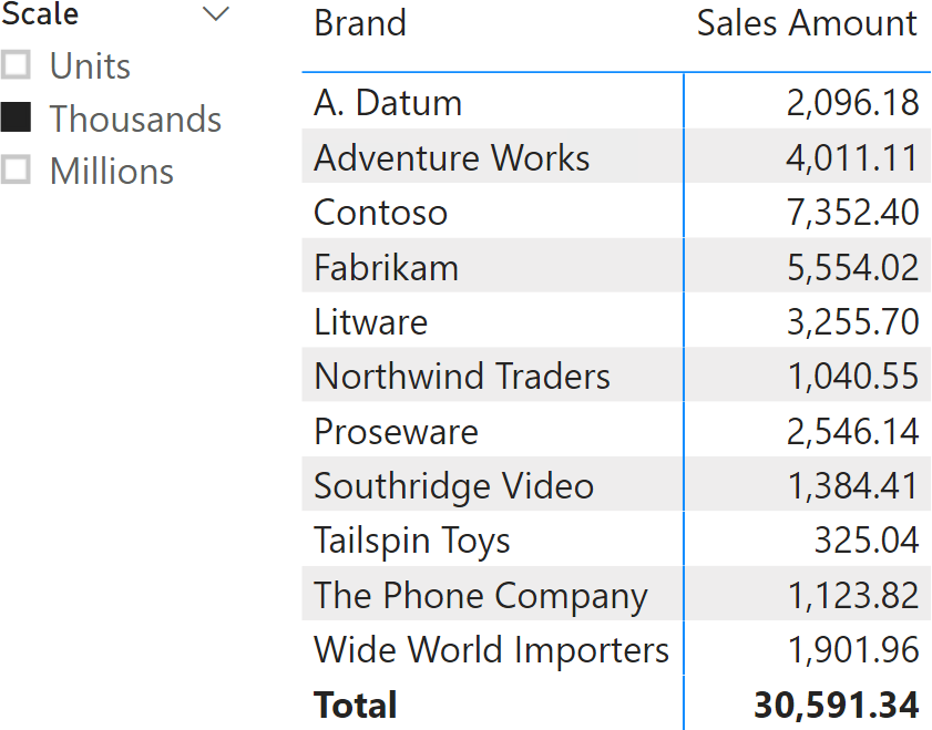
The user may need to be able to choose whether to show the Sales Amount measure as its actual value in dollars, or in thousands, or in millions. This is achieved with a slicer, as in the report visible in Figure 1. Though the real value of sales is around 30 million dollars, the measure shows it divided by one thousand as per the slicer selection.

The slicer requires a Scale table with the list of scales. That table includes two columns: one for the description to use in the slicer (Units, Thousands, Millions) and one to store the actual denominator to use when scaling the measure (1, 1,000, 1,000,000). The Scale calculated table can be created using the DATATABLE function:

Scale = 
DATATABLE (
    "Scale", STRING,
    "Denominator", INTEGER,
    {
        { "Units", 1 },
        { "Thousands", 1000 },
        { "Millions", 1000000 }
    }
)

Using the Sort by Column feature to sort Scale by the Denominator column is a best practice.

The Sales Amount measure scales down the result based on the denominator obtained by the current selection in the Scale[Denominator] column:

Sales Amount :=
VAR RealValue =
    SUMX ( Sales, Sales[Quantity] * Sales[Net Price] )
VAR Denominator =
    SELECTEDVALUE ( Scale[Denominator], 1 )
VAR Result =
    DIVIDE ( RealValue, Denominator )
RETURN
    Result

It is worth noting that despite the slicer being based on the Scale[Scale] column, that column also cross-filters the Scale[Denominator] column. Therefore, SELECTEDVALUE can query the Scale[Denominator] column directly.

If multiple measures must be scaled based on the same slicer, it might be convenient to define a measure returning the denominator value, instead of repeating the same code snippet in every measure that needs to follow the slicer selection:

Scale Denominator :=
SELECTEDVALUE ( Scale[Denominator], 1 )

Gross Sales :=
DIVIDE (
    SUMX ( Sales, Sales[Quantity] * Sales[Unit Price] ),
    [Scale Denominator] 
)

Total Cost :=
DIVIDE (
    SUMX ( Sales, Sales[Quantity] * Sales[Unit Cost] ),
    [Scale Denominator] 
)

Multiple independent parameters

If a calculation depends on multiple parameters, there could be multiple parameter tables in the model – one for each independent parameter.

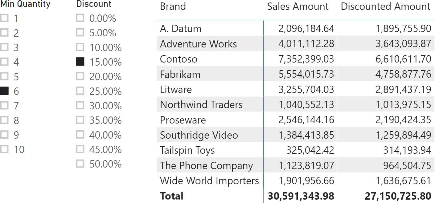
Imagine the simulation of a discount on orders: when the total number of items in a single order exceeds a given number of articles (Min Quantity parameter), the Discounted Amount measure applies the Discount parameter to the transaction. Users can simulate the effect of their choices on the historical data by using the slicers, as shown in Figure 2.

The implementation of the Discounted Amount measure first prepares a table in the Orders variable including the quantity and amount of each order. The result is obtained by iterating over the table in Orders, applying the discount to each individual order if the total quantity exceeds the defined boundary:

# Quantity :=
SUM ( Sales[Quantity] )

Discounted Amount := 
VAR MinQty =
    SELECTEDVALUE ( 'Min Quantity'[Min Quantity], 1 )
VAR Disc =
    SELECTEDVALUE ( Discount[Discount], 0 )
VAR Orders =
    ADDCOLUMNS (
        SUMMARIZE ( Sales, Sales[Order Number] ),
        "@Qty", [# Quantity],
        "@Amt", [Sales Amount]
    )
VAR Result =
    SUMX (
        Orders,
        IF (
            [@Qty] >= MinQty,
            ( 1 - Disc ) * [@Amt],
            [@Amt]
        )
    )
RETURN
    Result

By using multiple parameter tables, the parameters are independent from each other. In other words, a user can choose any combination of the two parameters, and the selection made in one parameter slicer does not affect the values available in other parameter slicers. In order to apply restrictions to the available combinations of parameters in different slicers, it is necessary to implement the multiple dependent parameters pattern.

Multiple dependent parameters

If a calculation depends on multiple parameters with limited available options, then a single table with one column for each parameter can store one row for each valid combination of the parameter values.

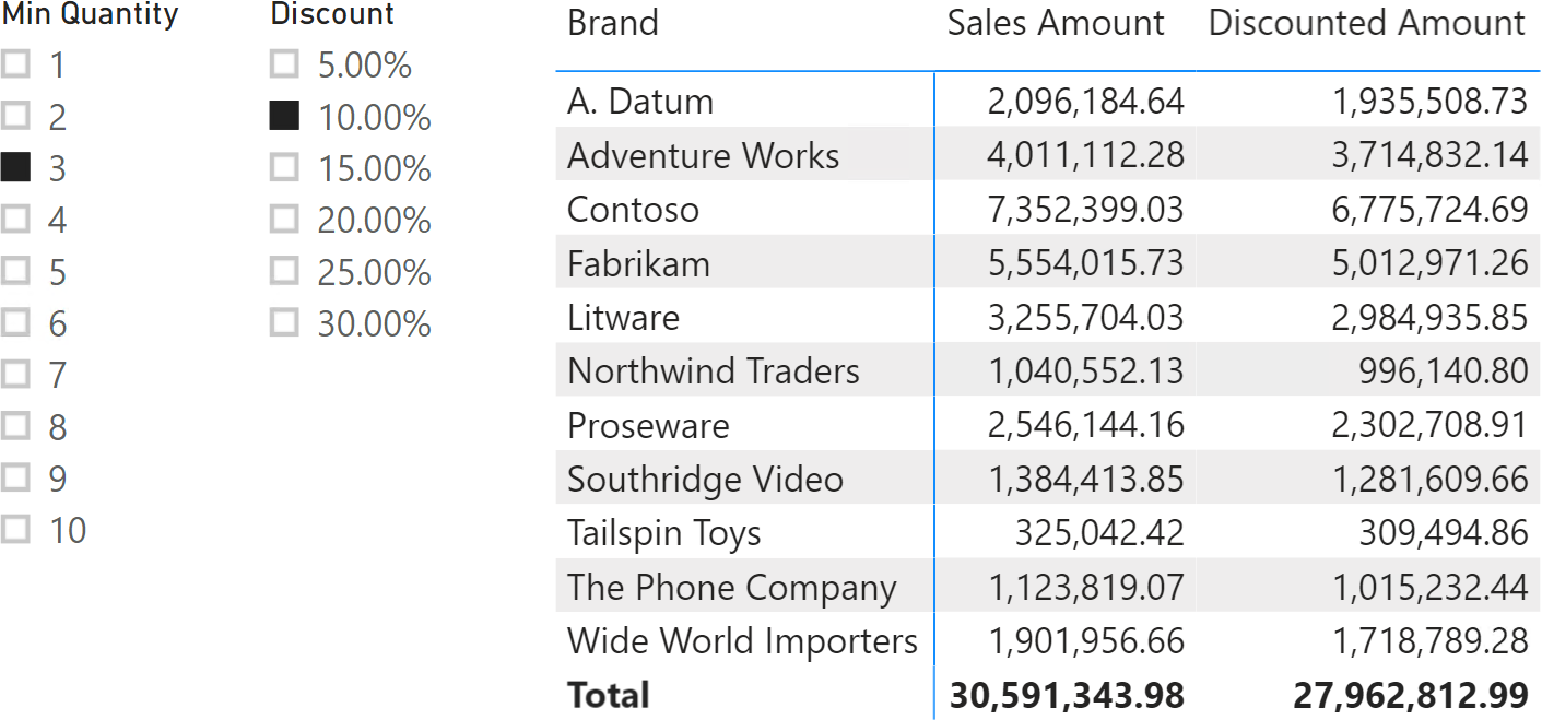
Imagine the scenario of the “Multiple independent parameters” pattern with two parameters: Min Quantity and Discount. The additional requirement is that the discount percentage cannot be greater than 10 times the Min Quantity. In other words, if a user selects 3 for Min Quantity, the maximum Discount available is 30%.

When the user makes a selection in the Min Quantity slicer, the Discount slicer only shows allowed percentage values according to the Min Quantity selected. Figure 3 shows an example of this scenario.

The Discounted Amount measure is identical to the measure used for the multiple dependent parameters example – it prepares a table in the Orders variable that includes the quantity and amount of each order, and then performs the proper calculation by iterating over the table in Orders:

# Quantity :=
SUM ( Sales[Quantity] )

Discounted Amount := 
VAR MinQty =
    SELECTEDVALUE ( Discount[Min Quantity], 1 )
VAR Disc =
    SELECTEDVALUE ( Discount[Discount], 0 )
VAR Orders =
    ADDCOLUMNS (
        SUMMARIZE ( Sales, Sales[Order Number] ),
        "@Qty", [# Quantity],
        "@Amt", [Sales Amount]
    )
VAR Result =
    SUMX (
        Orders,
        IF (
            [@Qty] >= MinQty,
            ( 1 - Disc ) * [@Amt],
            [@Amt]
        )
    )
RETURN
    Result

The Discount table contains both parameters in the Discount[Min Quantity] and Discount[Discount] columns. The Discount table must only include rows corresponding to valid combinations of Min Quantity and Discount. The following definition of the Discount calculated table only generates combinations where the Discount percentage is less than or equal to 10 times the Min Quantity:

Discount =
VAR Discounts =
    SELECTCOLUMNS ( GENERATESERIES ( 0, 19, 1 ), "Discount", [Value] / 20 )
VAR Quantities =
    SELECTCOLUMNS ( GENERATESERIES ( 1, 10, 1 ), "Min Quantity", [Value] )
RETURN
    GENERATE (
        Quantities,
        FILTER (
            Discounts,
            [Discount] <= [Min Quantity] / 10
        )
    )

The Discount table does not include combinations such as 3 for Min Quantity and 50% for Discount. Therefore, when the Min Quantity slicer selects 3, the Discount slicer only shows values less than or equal to 30%. The relationship between two or more parameters is implicitly found in the Discount table and directly affects the slicers through cross-filtering.

Selecting top N products dynamically

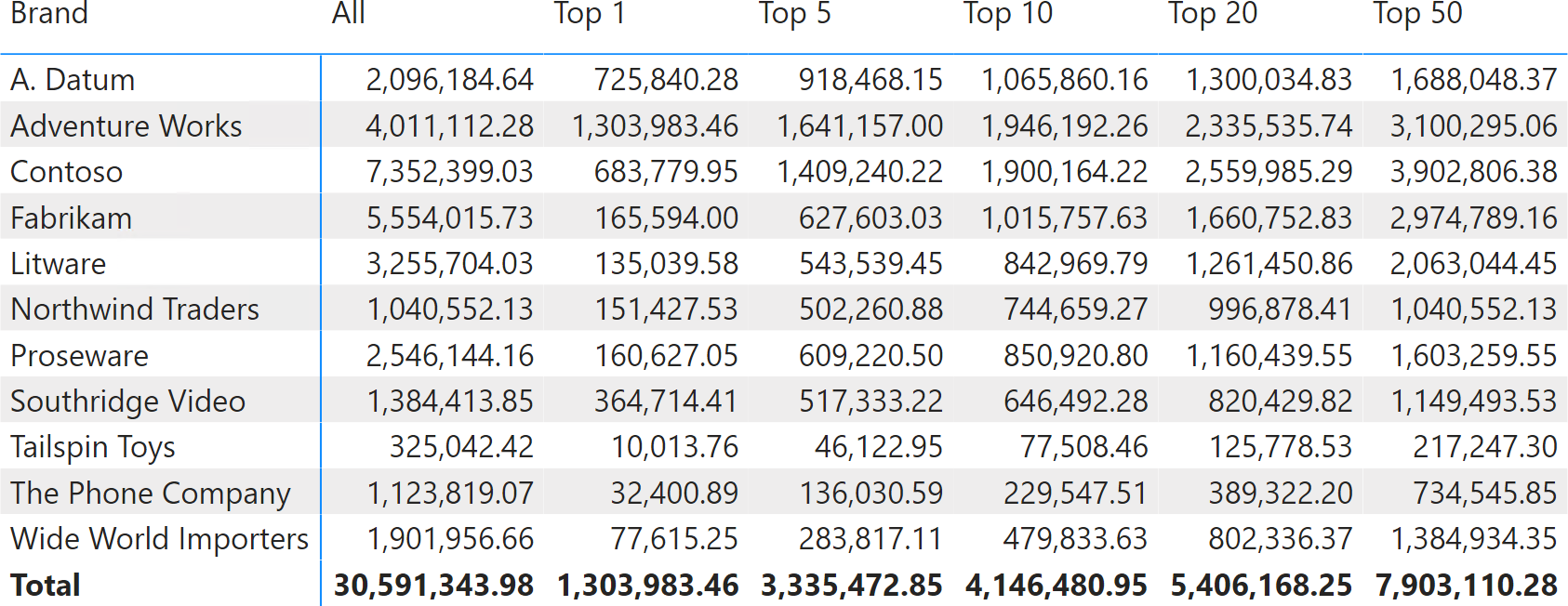
Imagine needing a report like the one in Figure 4, where each column filters a different number of products with the highest Sales Amount. Each column shows the Sales Amount of only the top N products, where N is determined by the column header. In this case, each visible name of the TopN parameter is mapped to a different number, used as the parameter value in the Top Sales measure.

This visualization is hard to obtain in Power BI, because the Top N visual-level filter can only be applied once in one visual. In this case, every column has a different parameter for the TOPN function used in the Top Sales measure.

The parameter table requires two columns: one for the visible name (TopN Products) that contains the description of the parameter, and the other column (TopN) is a number corresponding to both the result of the parameter selection and the sort order of the TopN Products values.

The TopN Filter calculated table can be defined with the following code:

TopN Filter =
ADDCOLUMNS (
    SELECTCOLUMNS ( 
        { 0, 1, 5, 10, 20, 50 }, 
        "TopN", [Value] 
    ),
    "TopN Products", IF (
        [TopN] = 0,
        "All",
        "Top " & [TopN]
    )
)

The Top Sales measure uses the selected value to filter the number of top products by evaluating the Sales Amount measure:

Top Sales :=
VAR TopNvalue =
    SELECTEDVALUE ( 'TopN Filter'[TopN], 0 )
VAR TopProducts =
    TOPN (
        TopNvalue,
        'Product',
        [Sales Amount]
    )
VAR AllSales = [Sales Amount]
VAR TopSales =
    CALCULATE (
        [Sales Amount],
        KEEPFILTERS ( TopProducts )
    )
VAR Result =
    IF (
        TopNvalue = 0,
        AllSales,
        TopSales
    )
RETURN
    Result

GENERATESERIES

Returns a table with one column, populated with sequential values from start to end.

GENERATESERIES ( <StartValue>, <EndValue> [, <IncrementValue>] )

DATATABLE

Returns a table with data defined inline.

DATATABLE ( <name>, <type> [, <name>, <type> [, … ] ], <data> )

SELECTEDVALUE

Returns the value when there’s only one value in the specified column, otherwise returns the alternate result.

SELECTEDVALUE ( <ColumnName> [, <AlternateResult>] )

TOPN

Returns a given number of top rows according to a specified expression.

TOPN ( <N_Value>, <Table> [, <OrderBy_Expression> [, [<Order>] [, <OrderBy_Expression> [, [<Order>] [, … ] ] ] ] ] )