Parent-child hierarchies are often used to represent charts of accounts, stores, salespersons and such. Parent-child hierarchies have a peculiar way of storing the hierarchy in the sense that they have a variable depth. In this pattern we show how to use parent-child hierarchies to show budget, actual and forecast values in a report using both a chart of accounts and a geographic hierarchy.

Introduction

In the parent-child pattern the hierarchy is not defined by the presence of columns in the table of the original data source. The hierarchy is based on a structure where each node of the hierarchy is related to the key of its parent node. For example,  Figure 1 shows the first few rows of a parent-child hierarchy that defines a geographic structure for sales.

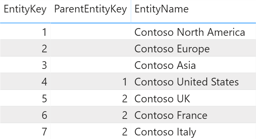
Based on this data structure, we need to display a hierarchy showing Contoso United States under Contoso North America, as shown in Figure 2.

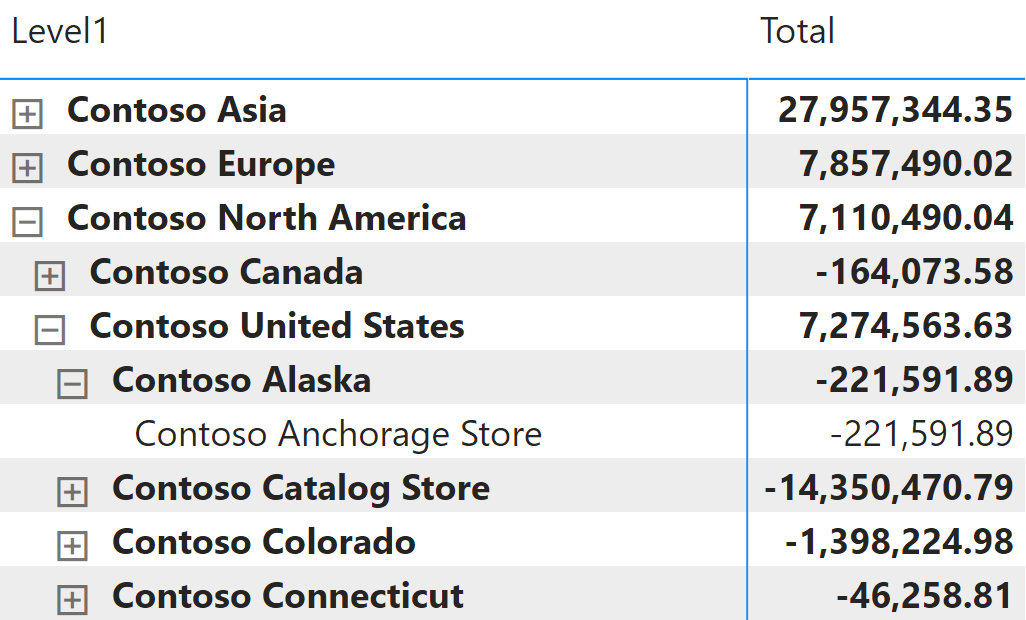
The parent-child pattern implements some sort of self-join of the table containing the entities, which is not supported in Tabular. Because of their nature, parent-child hierarchies may also have a variable depth: the number of levels traversing the hierarchy top to bottom can be different depending on the navigated path. For these reasons, a parent-child hierarchy should be implemented following the technique described in this pattern.

Parent-child hierarchies are often used with charts of accounts. In this case, the nodes also define the sign to use to aggregate a value to its parent. The chart of accounts in Figure 3 shows expenses that are subtracted from the total – despite the numbers displayed being all positive – whereas incomes are added.

The DAX expressions aggregating data over a parent-child hierarchy must consider the sign used to aggregate data at lower level of a hierarchy node.

Basic parent-child pattern

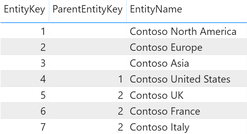
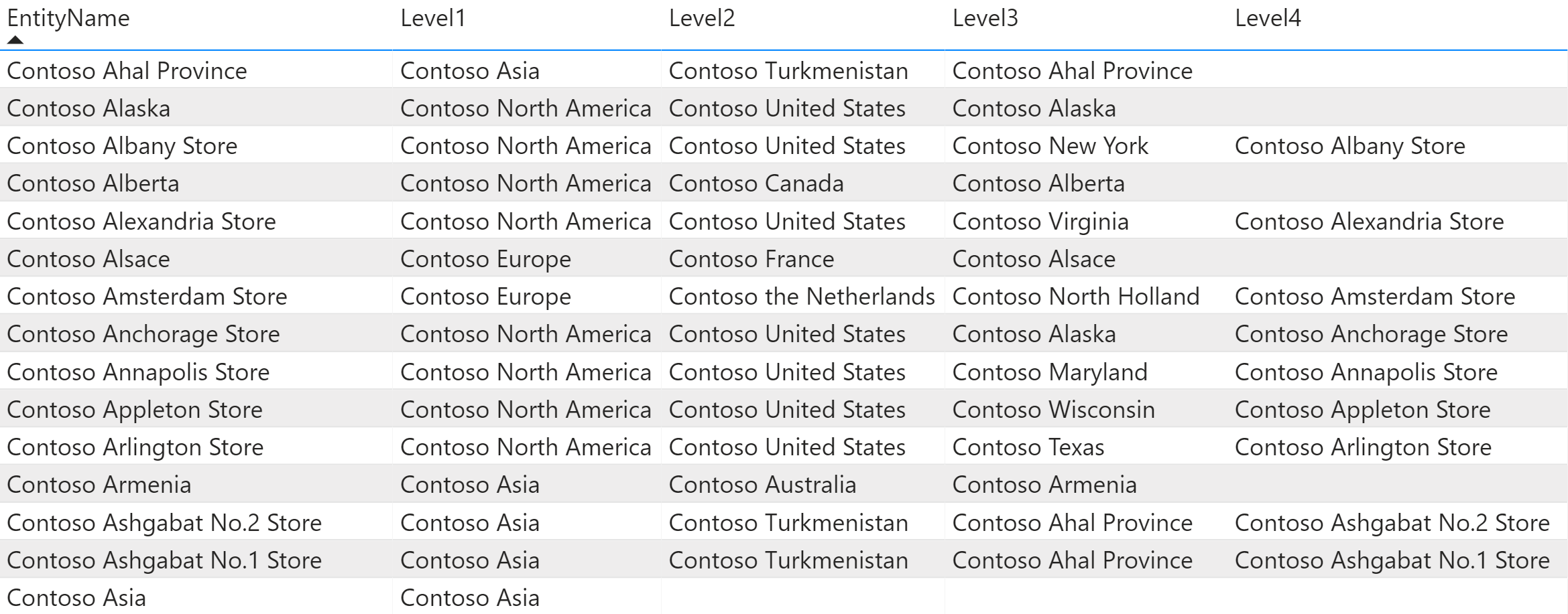
Neither hierarchies of variable depth nor self-joins are directly supported in a Tabular model. The first step in handling parent-child hierarchies is to flatten the hierarchical structure to a regular hierarchy made up of one column for each possible level of the hierarchy. We must move from the data structure of Figure 4 to that of Figure 5. In Figure 4 we only have the three columns required to define a parent-child hierarchy.

The full expansion of the parent-child hierarchy in this example requires four levels. Figure 5 shows that there is one column for each level of the hierarchy, named Level1 to Level4. The number of columns required depends on the data, so it is possible to add additional levels to accommodate for future changes in the data.

The first step is to create a technical column called EntityPath by using the PATH function:

EntityPath = 
PATH ( Entity[EntityKey], Entity[ParentEntityKey] )

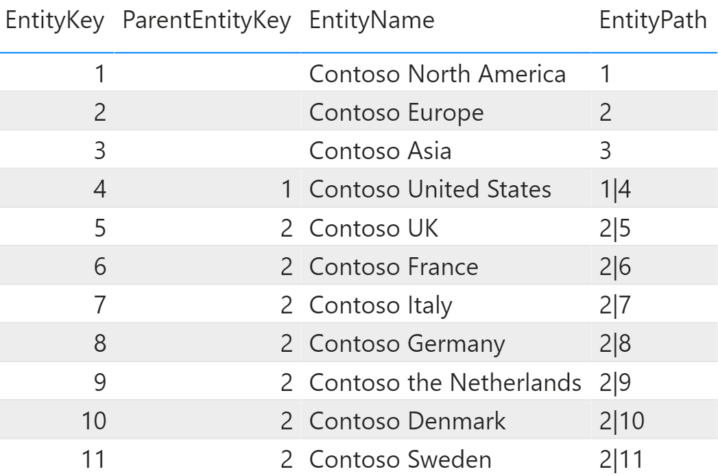
The EntityPath column contains the full path to reach the node corresponding to the row of the table, as shown in Figure 6. This technical column is useful to define the Level columns.

The code for all the Level columns is similar, and only differs in the value assigned to the LevelNumber variable. This is the code for the Level1 column:

Level1 =
VAR LevelNumber = 1
VAR LevelKey = PATHITEM ( Entity[EntityPath], LevelNumber, INTEGER )
VAR LevelName = LOOKUPVALUE ( Entity[EntityName], Entity[EntityKey], LevelKey )
VAR Result = LevelName
RETURN
    Result

The other columns have a different name and a different value assigned to LevelNumber, corresponding to the relative position of their level in the hierarchy. Once all the Level columns are defined, we hide them and create a regular hierarchy in the table that includes all of them – all the Level columns. Only exposing these columns through a hierarchy is important in order to make sure they are used in properly by the user navigating a report.

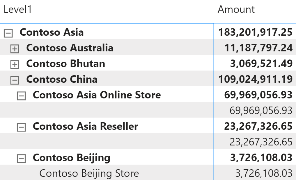
If used straight in a report, the hierarchy still does not provide an optimal result. Indeed, all the levels are always shown, even though they might contain no value. Figure 7 shows a blank row under Contoso Asia Online Store, even though the Level4 column for that node is blank – thus meaning that the node can be expanded only three levels, not four.

To hide the unwanted rows, for each row we must check whether the current level is available by the visited node. This can be accomplished by checking the depth of each node. We need a calculated column in the hierarchy table containing the depth of the node defined by each row:

Depth = 
PATHLENGTH ( Entity[EntityPath] )

We need two measures: EntityRowDepth returns the maximum depth of the current node, whereas EntityBrowseDepth returns the current depth of the matrix by leveraging the ISINSCOPE function:

EntityRowDepth := 
MAX ( Entity[Depth] )

EntityBrowseDepth :=
    ISINSCOPE ( Entity[Level1] )
    + ISINSCOPE ( Entity[Level2] )
    + ISINSCOPE ( Entity[Level3] )
    + ISINSCOPE ( Entity[Level4] )

Finally, we use these two measures to blank out the result if the EntityRowDepth is greater than the browsing depth:

Sum Amount := 
SUM ( StrategyPlan[Amount] )

Total Base := 
VAR Val = [Sum Amount]
VAR EntityShowRow =
    [EntityBrowseDepth] <= [EntityRowDepth]
VAR Result =
    IF ( EntityShowRow, Val )
RETURN
    Result

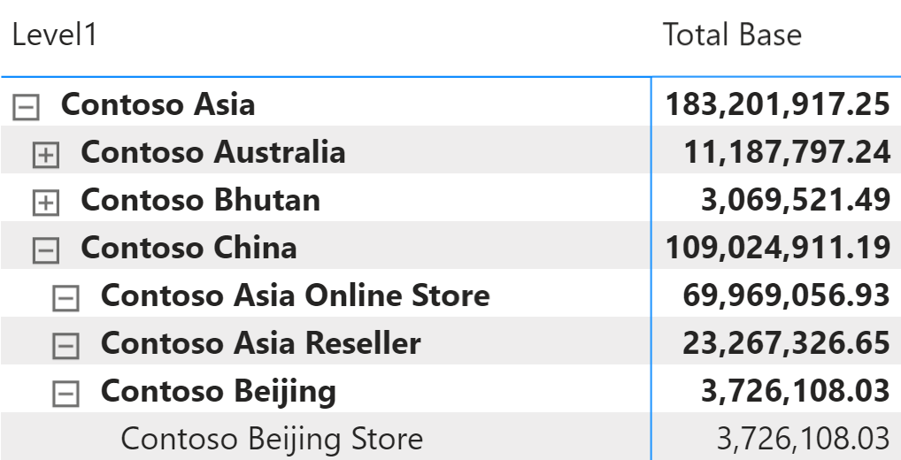
The report obtained by using the Total Base measure no longer contains rows with an empty description, as shown in Figure 8.

The same pattern must be applied to any measure that could be reported by using the parent-child hierarchy.

Chart of accounts hierarchy

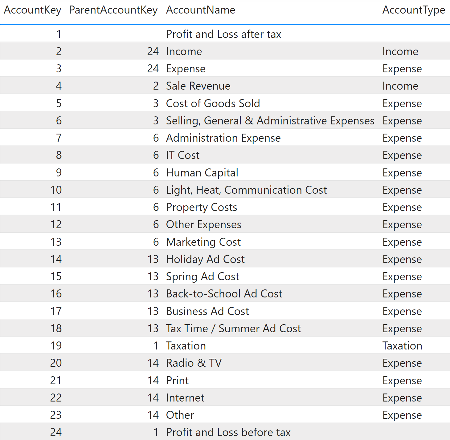
The Chart of accounts pattern is a variation of the basic Parent-child hierarchy pattern, where the hierarchy is also used to drive the calculations. Each row in the hierarchy is tagged as either Income, Expense or Taxation. Incomes need to be summed, whereas expenses and taxation must be subtracted from the total. The Figure 9 shows the content of the table containing the hierarchy items.

The implementation is similar to the parent-child pattern, grouping the calculation by AccountType and applying the proper sign to the calculation depending on the value of AccountType:

Total :=
VAR Val =
    SUMX (
        SUMMARIZE ( StrategyPlan, Account[AccountType] ),
        VAR SignToUse =
            IF ( Account[AccountType] = "Income", +1, -1 )
        VAR Amount = [Sum Amount] 
        RETURN
            Amount * SignToUse
    )
VAR AccountShowRow = [AccountBrowseDepth] <= [AccountRowDepth]
VAR EntityShowRow = [EntityBrowseDepth] <= [EntityRowDepth]
VAR Result =
    IF ( AccountShowRow && EntityShowRow, Val )
RETURN
    Result

The Total measure can use both parent-child hierarchies: the hierarchy defined in the Entity table – shown in the previous example – and the hierarchy defined in the Account table, which is the subject of this section.

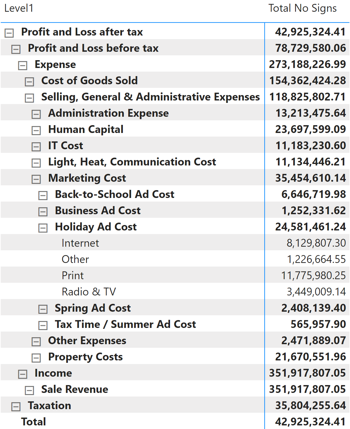
The formula in Total returns the right result for each node of the hierarchy. However, in these types of reports it is commonly requested that the numbers be shown as positive despite being expenses. The requirement can be fulfilled by changing the sign of the result at the report level. The following Total No Signs measure implements the calculation this way: It first determines the sign to use for the report, and then it changes the sign of the result in order to show expenses as positive numbers, even though they are internally managed as negative numbers:

Total No Signs = 
VAR BrowseLevel = [AccountBrowseDepth]
VAR AccountName =
    SWITCH (
        BrowseLevel,
        1, SELECTEDVALUE ( Account[Level1] ),
        2, SELECTEDVALUE ( Account[Level2] ),
        3, SELECTEDVALUE ( Account[Level3] ),
        4, SELECTEDVALUE ( Account[Level4] ),
        5, SELECTEDVALUE ( Account[Level5] ),
        6, SELECTEDVALUE ( Account[Level6] ),
        7, SELECTEDVALUE ( Account[Level7] )
    )
VAR AccountType =
    LOOKUPVALUE ( Account[AccountType], Account[AccountName], AccountName )
VAR ValueToShow = [Total]
VAR Result =
    IF ( AccountType IN { "Expense", "Taxation" }, -1, +1 ) * ValueToShow
RETURN
    Result

The report obtained using Total No Signs is visible in Figure 10.

The pattern shown above works fine if the chart of accounts contains the AccountType column, which defines each item as being either an income or an expense. Sometimes the chart of accounts has a different way of defining the sign to use. For example, there could be a column defining the sign to use when aggregating an account to its parent. This is the case of the Operator column shown in Figure 11.

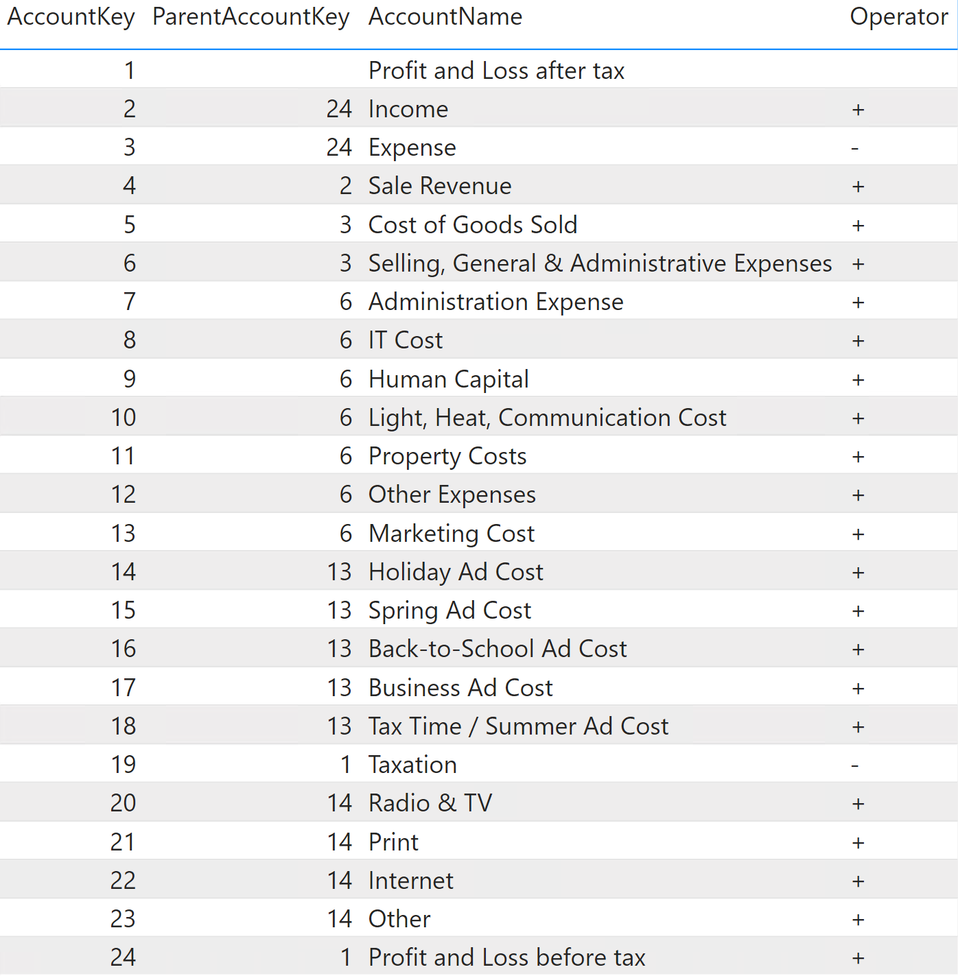
In this case, the code to author is more complex. We need one column for each level of the hierarchy, stating how that account needs to be shown when aggregated at any given level of the hierarchy. A single account can be aggregated at one level with a plus, but at a different level with a minus.

These columns need to be built from the bottom of the hierarchy. In this example we need seven columns because there are seven levels. The column indicates the sign to use when aggregating that specific item of the hierarchy at the desired level. Figure 12 shows the result of the seven columns in this example.

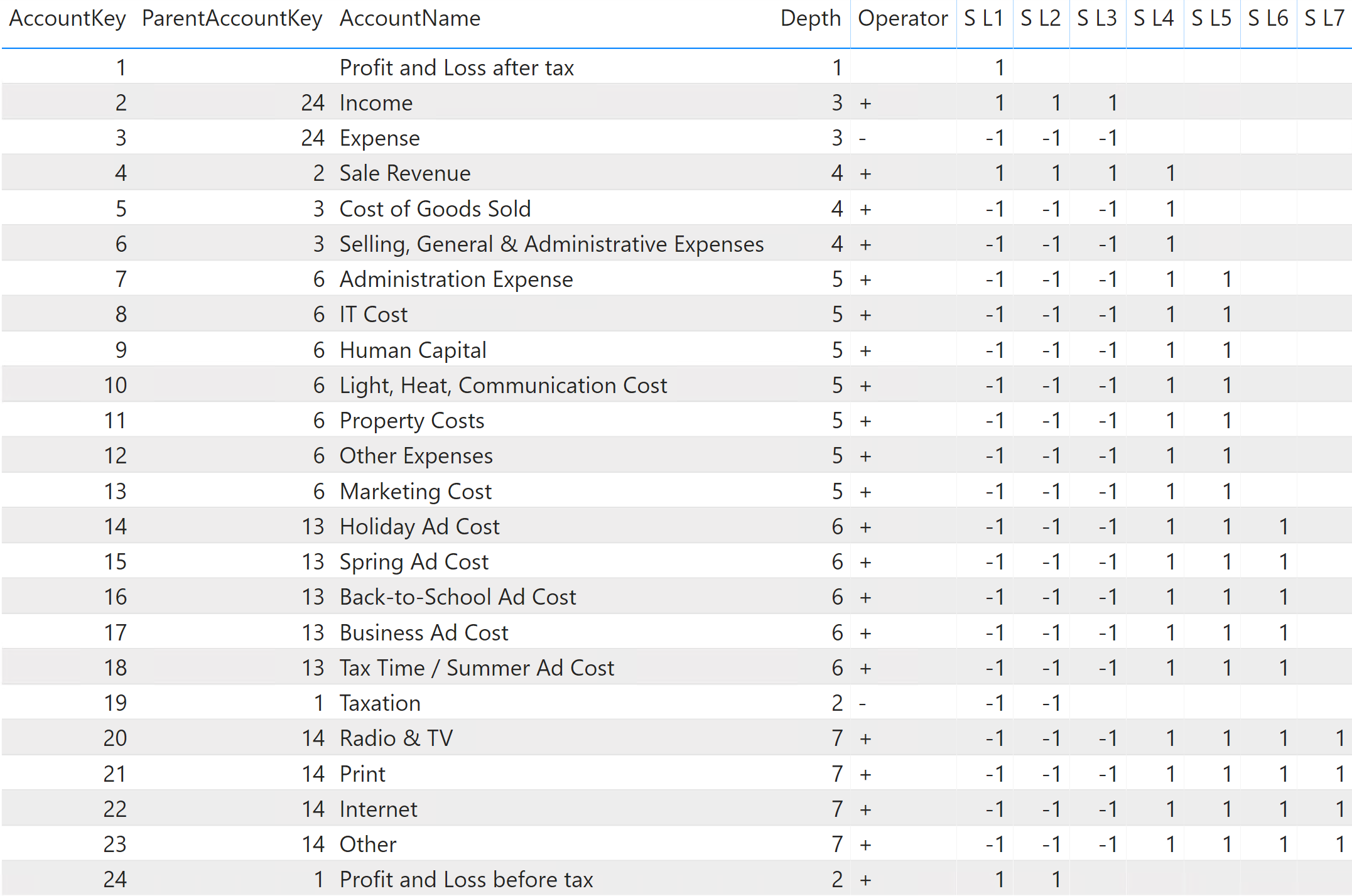
For instance, examine the rows with AccountKey 4 and 5: account 4 (Sale Revenue) must be summed when aggregated at levels 1, 2, 3 and 4, whereas it is not visible at other levels. Account 5 (Cost of Goods Sold) must be summed when aggregated at level 4, but it must be subtracted when aggregated at levels 1, 2, and 3.

The DAX formula computing the sign at each level starts from the most granular level –level 7 in our example. At this most granular level, the sign to use is just the operator converted into +1 or -1, for convenience in further calculations:

SignToLevel7 =
VAR LevelNumber = 7
VAR Depth = Account[Depth]
RETURN
    IF ( LevelNumber = Depth, IF ( Account[Operator] = "-", -1, +1 ) )

All the other columns (from level 1 to level 6) follow a similar pattern, though for each level the DAX expression must consider the sign at the more granular, adjacent level (stored in the PrevSign variable) and invert the result when that level shows a “-“ sign, as shown in the column for level 6:

SignToLevel6 =
VAR LevelNumber = 6
VAR PrevSign = Account[SignToLevel7]
VAR Depth = Account[Depth]
VAR LevelKey =
    PATHITEM ( Account[AccountPath], LevelNumber, INTEGER )
VAR LevelSign =
    LOOKUPVALUE ( Account[Operator], Account[AccountKey], LevelKey )
RETURN
    IF (
        LevelNumber = Depth,
        IF ( Account[Operator] = "-", -1, +1 ),
        IF ( LevelNumber < Depth, IF ( LevelSign = "-", -1, +1 ) * PrevSign )
    )

Once the level columns are ready, the Signed Total measure computing the total with custom signs is the following:

Signed Total :=
VAR BrowseDepth =
    MAX ( [AccountBrowseDepth], 1 )
VAR AccountShowRow = [AccountBrowseDepth] <= [AccountRowDepth]
VAR EntityShowRow = [EntityBrowseDepth] <= [EntityRowDepth]
VAR Result =
    IF (
        AccountShowRow && EntityShowRow,
        SWITCH (
            BrowseDepth,
            1, SUMX (
                VALUES ( Account[SignToLevel1] ),
                [Sum Amount] * Account[SignToLevel1]
            ),
            2, SUMX (
                VALUES ( Account[SignToLevel2] ),
                [Sum Amount] * Account[SignToLevel2]
            ),
            3, SUMX (
                VALUES ( Account[SignToLevel3] ),
                [Sum Amount] * Account[SignToLevel3]
            ),
            4, SUMX (
                VALUES ( Account[SignToLevel4] ),
                [Sum Amount] * Account[SignToLevel4]
            ),
            5, SUMX (
                VALUES ( Account[SignToLevel5] ),
                [Sum Amount] * Account[SignToLevel5]
            ),
            6, SUMX (
                VALUES ( Account[SignToLevel6] ),
                [Sum Amount] * Account[SignToLevel6]
            ),
            7, SUMX (
                VALUES ( Account[SignToLevel7] ),
                [Sum Amount] * Account[SignToLevel7]
            )
        )
    )
RETURN
    Result

We can compare the result of this last Signed Total measure with that of the previous Total measure in Figure 13.

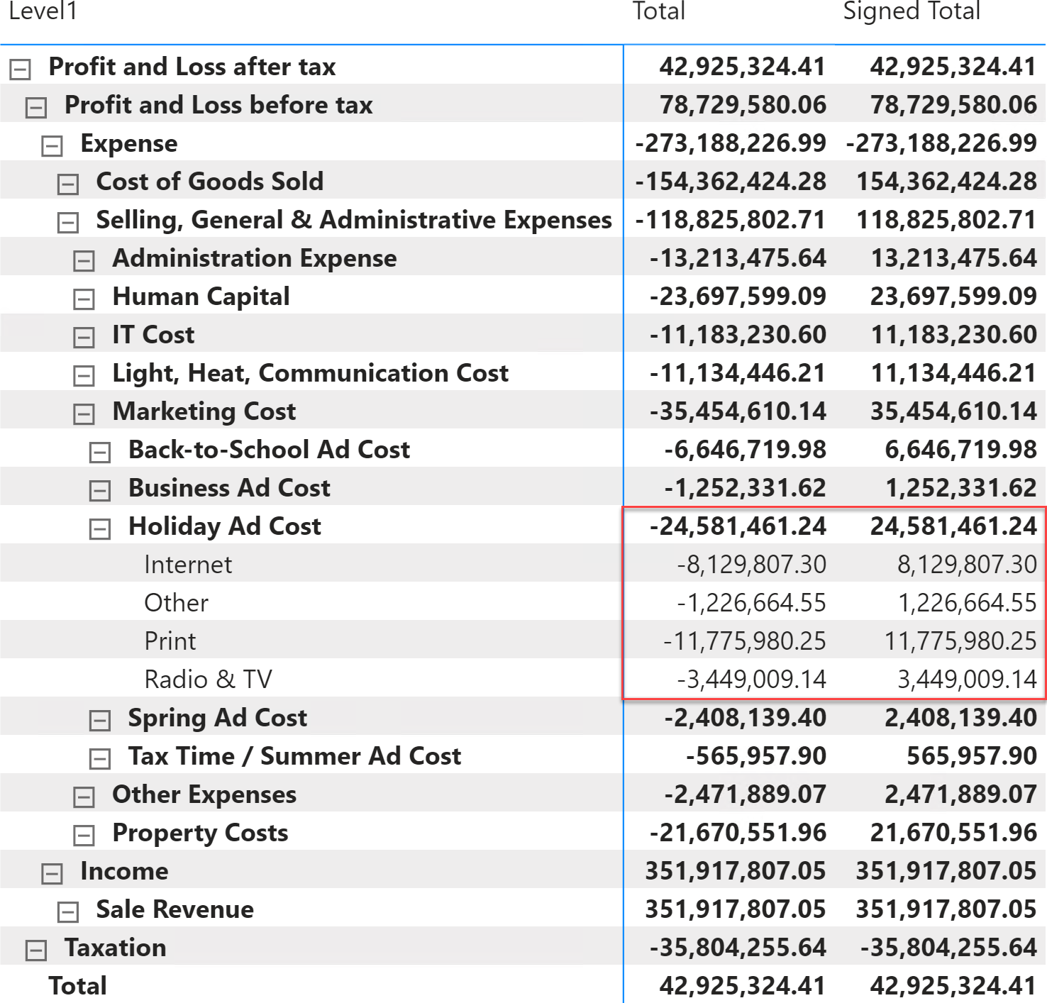
The amount for “Internet” is negative in Total, because it is an expense. However, in Signed Total the same row holds a positive number and it becomes negative only when it traverses the Expense node, which is aggregated to the parent with a minus sign.

Security pattern for a parent-child hierarchy

A common security requirement for parent-child hierarchies is to restrict the visibility to a node (or a set of nodes) including all of its children. In that scenario, the PATHCONTAINS function is useful.

By applying the following expression to a security role on the Account table, we limit the visibility to the node provided in the second argument of PATHCONTAINS. This way, all the children of the node are made visible to the user, because the node requested (2, corresponding to Income) is also part of the AccountPath value of all the children nodes:

PATHCONTAINS ( 
    Account[AccountPath],
    2  -- Key of Income
)

If we used the AccountKey column to limit the visibility, we would end up limiting the visibility to only one row and the user would not see the children nodes. By leveraging the path column, we can easily select multiple rows by including all the nodes that can be reached when traversing a path that includes the filtered node.

When the security role is active, the user can only see the nodes (and the values) included in the tree starting from the Income node, as shown in Figure 14.

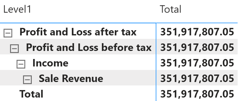
The nodes above the Income node (Level3) no longer consider other children nodes in the Total measure. In case this is misleading in the report, consider removing the initial levels from the report (in this case Level1 and Level2) or using different descriptions of the nodes in Level1 and Level2 in order to better explain the result.

It is worth noting that the security role defined by using PATHCONTAINS may slow down the performance if used with a hierarchy with thousands of nodes. The expression in the role security must be evaluated for every node of the hierarchy when the end user opens a connection, and PATHCONTAINS can be expensive if it is applied to thousands of rows or more.

PATH

Returns a string which contains a delimited list of IDs, starting with the top/root of a hierarchy and ending with the specified ID.

PATH ( <ID_ColumnName>, <Parent_ColumnName> )

ISINSCOPE

Returns true when the specified column is the level in a hierarchy of levels.

ISINSCOPE ( <ColumnName> )

PATHCONTAINS

Returns TRUE if the specified Item exists within the specified Path.

PATHCONTAINS ( <Path>, <Item> )